Accuracy on Non-stationary Data Streams

We measured the statistical distance between the underlying distribution of various non-stationary data streams and the distributions estimated by using Sketch and its alternatives, oKDE and SPDTw. Furthermore, we analyze the change in the statistical distance by using the harmonic oscillator model.

The data streams with three different concept drifts—incremental concept drift, sudden concept drift, and blip concept drift—are used in these experiments. First, we estimate the PDFs for data streams with incremental concept drift to test if the estimated PDFs adapt well to concept drifts. Second, we estimate the PDFs for data streams with sudden concept drift to test if the estimated PDFs forget previous concept quickly. Third, we estimate the PDFs for data streams with blip concept drift to provide an insight into the stability of the estimated PDF when outlier occurs.

Incremental Concept Drift

Incremental concept drift is defined as the case where the distribution of the data stream changes incrementally. The underlying distribution is a normal distribution whose mean value moves at a constant speed, i.e., $\mathcal{N}(x(t), 1)$ where

$x(t) = \begin{cases} 0, & t \leq t_1 \\ v_1 \cdot (t - t_1), & t > t_1 \\ \end{cases}$

$t$ is the timestamp of data, $t_1 = 300$, and $v_1 = 0.01$.

infographic

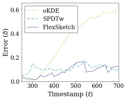
Upper figures show how the statistical distance between the PDFs estimated using different algorithms and the underlying distribution of the data stream with incremental concept drift changes over time. The statistical distances of SPDTw and Sketch are saturated at 0.14 and 0.11, respectively, but that of oKDE is saturated at 0.58.

We use the lag as a metrics indicating how well the estimated PDF adapts to the data stream with incremental concept drift. A lag is defined as the ratio between the restoring coefficient and the resistance coefficient of harmonic oscillator model, i.e., $c/k$. If incremental concept drift occurs at a constant speed, $\ddot{D_\Delta} = 0$ in harmonic oscillator model for large $t$. In this case, the magnitudes of the restoring and resistance forces are the same—we refer to it as the dynamic equilibrium in the space of $D_\Delta$. Thus, the lag is represented as follows:

$\label{eq:ratiorr} \frac{c}{k} = \frac{D_\Delta}{\dot{D_\Delta}}$

According to this equation, $c/k$ is directly proportional to $D_\Delta$ as $\dot{D_\Delta}$ is approximately constant. This is why we call $c/k$ the lag.

infographic

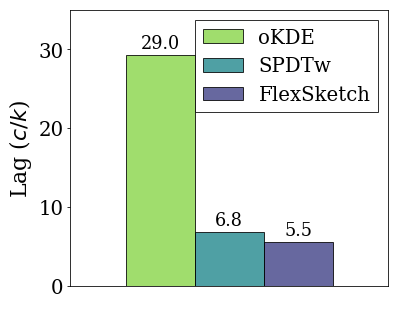
Upper diagram shows the lags for various algorithms. The PDF estimated using Sketch is 5.3$\times$ and 1.2$\times$ better adapted to the data stream than that obtained using oKDE and SPDTw, respectively, when incremental concept drift occurs.

Sudden Concept Drift

Sudden concept drift is defined as the case where the distribution of the data stream changes suddenly. The underlying distribution is a normal distribution whose mean value moves suddenly, i.e., $\mathcal{N}(x(t), 1)$ where

$x(t) = \begin{cases} 0, & t < t_1 \\ x_1, & t \geq t_1 \\ \end{cases}$

$t$ is the timestamp of data, $t_1 = 300$, and $x_1 = 5$.

infographic

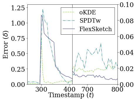
Upper figures show how the statistical distance between the PDFs estimated using different algorithms and the underlying distribution of the data stream with sudden concept drift changes over time.

The solution of the harmonic oscillator model for $D_\Delta$, under the assumption of over-damped oscillation, i.e., $(c/2)^2 > k$, is as follows:

$D_\Delta(t) = \underbrace{A_1 e^{-(\lambda + \omega) t}}_{\text{Short-lived term}} + \underbrace{A_2 e^{- (\lambda - \omega) t}}_{\text{Long-lived term}}$

where $\lambda = c/2$ and $\omega = \sqrt{\lambda^2 - k}$. In the experiment for incremental concept drift, we obtain the $c/k$. By using this, we select $\lambda$ and $\omega$ so that this equation has the best fit to the figure of statistical distance for timestamp.

We can measure how quickly the estimated PDF can forget the previous concept in a short and long term through the changes in statistical distances: half-life and lifetime, respectively. The half-life is a metric indicating how fast the estimated PDF adapts to the data stream in the short term. It is the time required for a statistical distance at $t_1$ to reduce to half its initial value. The half-life is defined as followings:

$t_{1/2} = D_\Delta^{-1} \Big({1}/{2} \cdot D_\Delta(t_1) \Big)$

The lifetime is a metric indicating how long the contribution of the past data stays. It is the time required for a long-lived term of $D_\Delta(t)$ to reduce to ${1}/{e}$ its initial value. The lifetime is defined as followings:

$\tau = (\lambda - \omega)^{-1}$

infographic

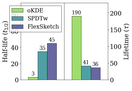
Upper figure shows the half-lives and lifetimes for each algorithms. The PDF estimated using Sketch is 0.066$\times$ and 0.78$\times$ better adapted to the data stream than that obtained using oKDE and SPDT, respectively when sudden concept drift occurs in the short term. Furthermore, the PDF estimated using Sketch is 5.2$\times$ and 1.1$\times$ better adapted to the data stream than that obtained using oKDE and SPDT, respectively, in the long term.

As shown in this experiment, oKDE adapts much faster than SPDTw and Sketch in the short term. However, oKDE adapts much slower than SPDTw and Sketch in the long term. Thus, we can conclude that oKDE produces unstable results and it is vulnerable to numerous concept drifts in the long term. Refer to the blip concept drift case for further discussions on outliers.

Blip Concept Drift

Blip concept drift is defined as the case where the distribution of data stream suddenly changes and returns to the original state in a short time. The underlying distribution is a normal distribution whose mean value moves as follows, i.e., $\mathcal{N}(x(t), 1)$ where

$x(t) = \begin{cases} x_1, & t_1 < t \leq t_1 + t_\epsilon \\ 0, & \text{otherwise} \\ \end{cases}$

$t_\epsilon$ is the duration of blip concept drift, $t_\epsilon = 3$, $x_1 = 5$, and $t_1 = 300$. Strictly, the blip concept drift is different from an outlier . However, the blip concept drift for a short period of time can be approximated to an outlier. Therefore, the behavior of the estimated PDF for blip concept drift over a short time can provide insight into the stability of the estimated PDF when an outlier occurs.

infographic

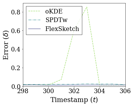
Upper figures show how the statistical distance between the PDFs estimated using different algorithms and the underlying distribution of data stream (at the origin) with blip concept drift changes over time. In this figure, the statistical distance of Sketch and SPDTw is increased only by 0.0050 and 0.0021, respectively, during blip concept drift, but the statistical distance of oKDE is increased by 0.84.

We use the volatility as a metric that measures how fast the estimated PDF moves for a short duration when blip concept drift occurs. The volatility is average velocity during blip concept drift. The volatility is defined as follows:

$\sigma = \frac{D_\Delta(t_1 + t_\epsilon) - D_\Delta(t_1)}{t_\epsilon}$

The lower the volatility, the more stable the estimated PDF, when accidental outliers are included in the data stream.

infographic

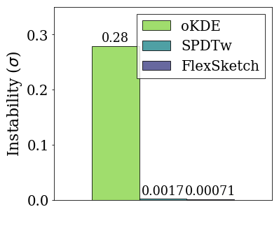
Upper figure shows the volatility for each algorithms. The PDF estimated using Sketch is 390$\times$ and 2.3$\times$ more stable than that obtained using oKDE and SPDTw, respectively, when blip concept drift occurs.

In this experiment, the volatility of Sketch is far lower than that of oKDE. This result is compatible with the experiment for sudden concept drift that shows the half-life of oKDE is much greater than that of Sketch.