Performance on Parameters

When the Sketch framework estimates the PDF for stationary and non-stationary data streams, appropriate parameters should be selected to achieve high update speed and accuracy with only a small amount of memory. Our experiment demonstrates that it is advantageous to set parameters so that they are analogous to traditional density estimation models as best as possible when estimating stationary data streams. Furthermore, our experiment shows that there is a trade-off between the accuracy and update speed when selecting parameters for estimating non-stationary data streams.

In this experiment, we observed the change in the three key metrics of Sketch—throughput of the update operation, statistical distance, and memory usage—when its parameters are modified. There are two types of synthetic data streams used for the density estimation. One is a stationary data stream of normal distribution $\mathcal{N}(0, 1)$ and the other is a non-stationary data stream whose mean constantly moves, i.e., $\mathcal{N}(v_1 \cdot t, 1)$ where $v_1 = 0.01$. The range of parameters in this experiments are as follows: from 2 to 10 for cmapNo, from 10 to 150 for thresholdPeriod, from 0.2 to 3.0 for decayFactor, and from 0.01 to 2.3 for rebuildThreshold.

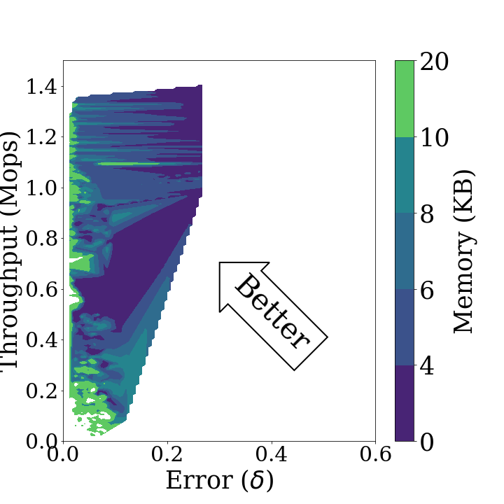
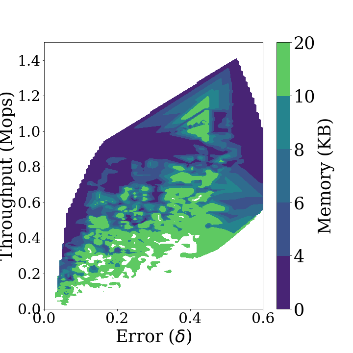
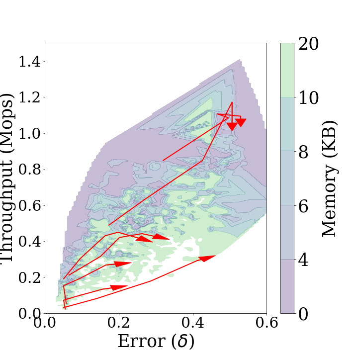
The performance diagram is defined as the three-dimensional representation of key metrics for Sketch over various parameters. First in the diagrams above show the performance diagrams for the stationary and non-stationary data streams of Sketch respectively. These diagrams demonstrate the throughput, statistical distance and memory usage that can be achieved by Sketch in each type of data stream. As the algorithm has better performance, the displayed area in the diagrams is shifted to the upper left. Second in the diagrams above shows that Sketch can achieve low statistical distance and high throughput at the same time using a small amount of memory if it estimates a stationary distribution. Figure 3b indicates that there is a trade-off between high accuracy and throughput when Sketch estimates a non-stationary data stream. Furthermore, in a non-stationary case, more memory usage is required to achieve the same throughput and accuracy as in a stationary case. When concept drift occurs, the performance diagram is distorted in a diamond shape, which indicates that overall performance is degraded.

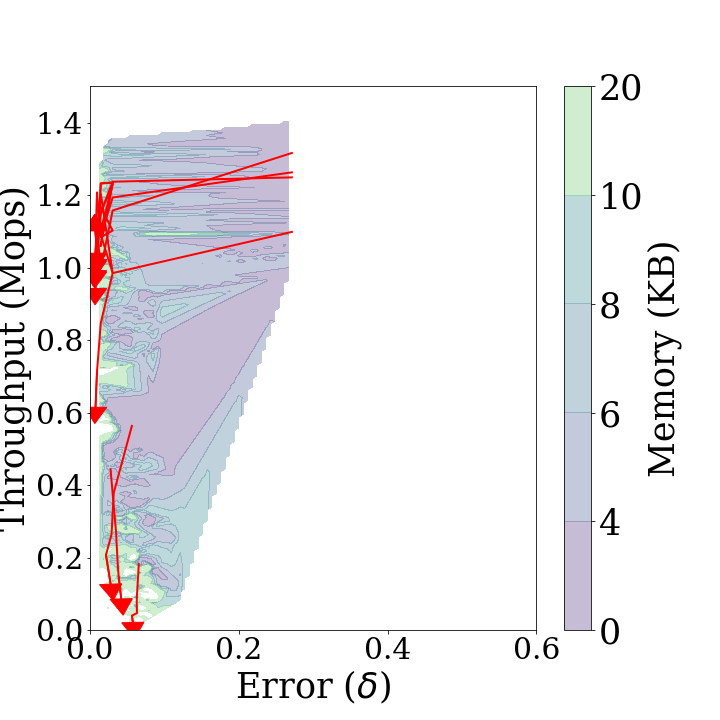
The performance trend is the trajectory arrows changing each parameter at a time while the others remain fixed. show the performance trends added on each performance diagram. In the figures, the longer the arrow, the more the performance changes. If the arrows are down right, the statistical distance increases and the throughput decreases as the parameters increase, which indicates that the performance of Sketch degrades in all respects. On the other hand, if the arrows are up right, it indicates that the statistical distance increases and the throughput increases as the parameters increase, thus being in a trade-off relationship. The up left arrow and the down left arrow are the opposite.

Stationary Case

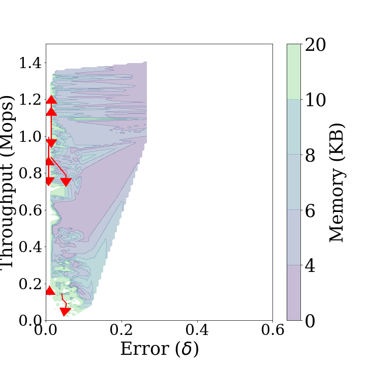
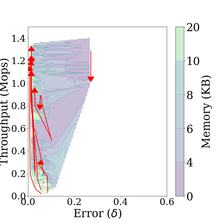
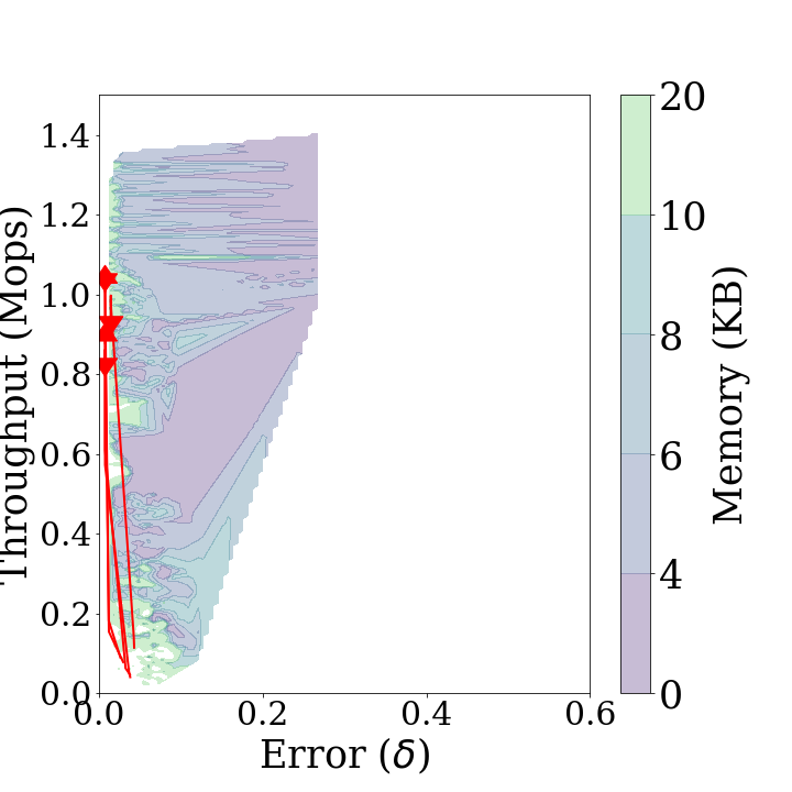
• cmapNo: First in the diagrams above shows the performance trends for cmapNo. These treands are downward arrows. They indicate that the statistical distance does not change and the thoughput decreases as cmapNo increases.
• thresholdPeriod: Second in the diagrams above shows the performance trends for thresholdPeriod. These trends are left upward arrows. They indicate that the statistical distance decreases and the throughput increases as thresholdPeriod increases. This is because the [Diagnose]{.smallcaps} is performed more rarely.
• decayFactor: Third in the diagrams above shows the performance trends for decayFactor. These trends are very short, random arrows. They indicate that the key metrics of Sketch are not affected by decayFactor.
• rebuildThreshold:Fourth in the diagrams above shows the performance trends for rebuildThreshold. These trends are right downward arrows. They indicate that the throughout increases and the statistical distance decreases as rebuildThreshold increases, owing to the same reason of thresholdPeriod.

In conclusion, it is advantageous to select thresholdPeriod and rebuildThreshold as large as possible to increase the throughput and decrease the statistical distance. cmapNo should be as small as possible. decayFactor had no influence on the results.

In evaluating the performance of the parameters, one must consider the stability of the estimated PDF when outliers occur as these diagrams use the mean statistical distance. If cmapNo is less than 3 or rebuildThreshold is less than 2.5, the statistical distance increases temporarily when an outlier accidentally occurs.

These results demonstrate that the use of solely the update operation, as in the traditional approach, is advantageous to the performance of estimation for a stationary data stream. If thresholdPeriod and rebuildThreshold are small, the majorUpdate operation is performed frequently. The majorUpdate operation adds a model representing the latest data stream to the data structure of Sketch. Consequently, the PDF estimated using Sketch is strongly dependent on the latest data, and its accuracy is compromised when estimating the distribution of a stationary data stream.

Non-stationary Case

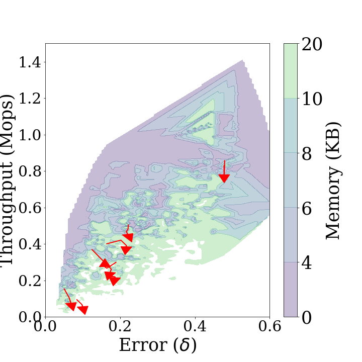
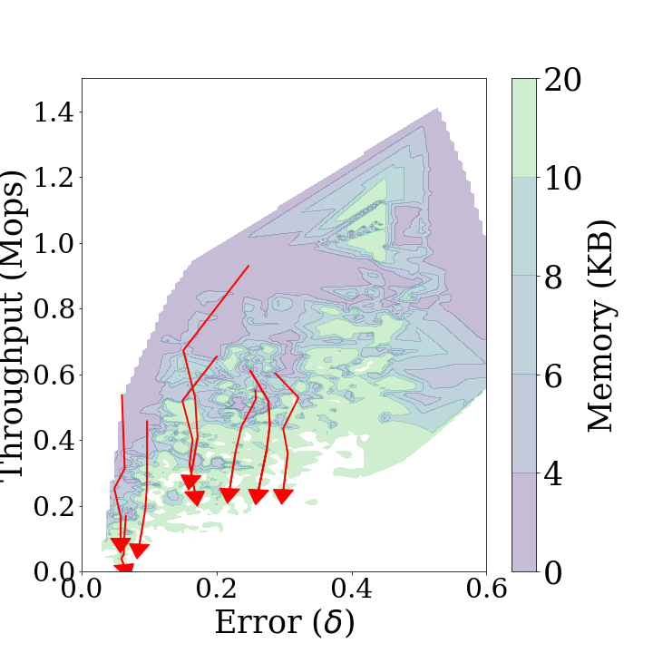
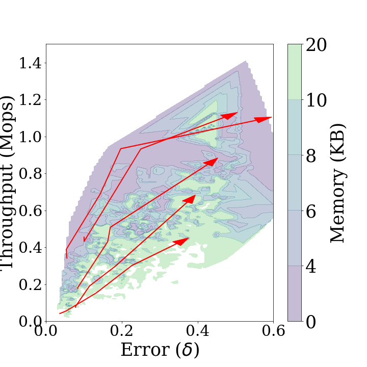
• cmapNo: First in the diagrams above shows the performance trends for cmapNo. These trends are downward arrows. They indicate that the statistical distance increases and the throughput decreases as cmapNo increases.
• thresholdPeriod: Second in the diagrams above shows the performance trends for thresholdPeriod. These trends are left upward arrows. They indicate that both the statistical distance and throughput increase as the thresholdPeriod increases. This is because the [Diagnose]{.smallcaps} and majorUpdate operation are performed more frequently.
• decayFactor: Third in the diagrams above shows the performance trends for decayFactor. These trends are leftward arrows. They indicate that the statistical distance decreases as decayFactor increases.
• thresholdPeriod: Fourth in the diagrams above shows the performance trends for rebuildThreshold. These trends are right upward arrows. They indicate that both the statistical distance and throughput increase as rebuildThreshold increases, owing to the same reason of thresholdPeriod.

In conclusion, for the selection of thresholdPeriod and rebuildThreshold, there is a trade-off between the statistical distance and throughput. cmapNo and decayFactor should be as small as possible.

This result is the opposite of the stationary case, and this indicates that, when the data stream is non-stationary, performing the update operation consisting of two different update operations (i.e., minorUpdate and majorUpdate) helps to improve its accuracy. This is because, with a smaller thresholdPeriod and rebuildThreshold, the use of two update operations has a significant influence on the accuracy.

Selection Rule

To perform density estimation with high throughput and accuracy for both stationary and non-stationary data streams, parameters should be selected to satisfy the following rules based on the results of the above experiments.

• cmapNo: 3 is the optimal value. We choose the smallest value so long as the value is not so small that the model happens to have an excessively high statistical distance accidentally.
• thresholdPeriod: We choose the largest value within the range that satisfies the requirements of accuracy and memory usage. The allowed range of thresholdPeriod should be determined experimentally. In all experiments, we select 30.
• decayFactor: 2.5 is the optimal value. We choose the highest value so long as the value is not so high that the model happens to have an excessively high statistical distance accidentally.
• thresholdPeriod: We choose the largest value within the range that satisfies the requirements of accuracy and memory usage. The range of rebuildThreshold should be determined experimentally. In all experiments, we select 0.4.